pandasをインストールしたのでデータをいじってみる

pandasをインストールしたのでデータをいじってみる
自分用の備忘録ですがよろしくお願いします。
CSVの読み込み
import pandas as pd
transaction = pd.read_csv('transaction_1.csv')
transaction.head()
     transaction_id   price         payment_date customer_id
0       T0000000113  210000  2019-02-01 01:36:57    PL563502
1       T0000000114   50000  2019-02-01 01:37:23    HD678019
2       T0000000115  120000  2019-02-01 02:34:19    HD298120
3       T0000000116  210000  2019-02-01 02:47:23    IK452215
4       T0000000117  170000  2019-02-01 04:33:46    PL542865
...             ...     ...                  ...         ...
縦に結合(concat)
import pandas as pd
transaction_1 = pd.read_csv('transaction_1.csv')
transaction_2 = pd.read_csv('transaction_2.csv')
transaction = pd.concat([transaction_1, transaction_2], ignore_index=True)
transaction.head()

print(len(transaction_1))#5000(レコード数)
print(len(transaction_2))#1786(レコード数)
print(len(transaction))  #6786(レコード数)
     transaction_id   price         payment_date customer_id
0       T0000000113  210000  2019-02-01 01:36:57    PL563502
1       T0000000114   50000  2019-02-01 01:37:23    HD678019
2       T0000000115  120000  2019-02-01 02:34:19    HD298120
3       T0000000116  210000  2019-02-01 02:47:23    IK452215
4       T0000000117  170000  2019-02-01 04:33:46    PL542865
...             ...     ...                  ...         ...
6781    T0000006894  180000  2019-07-31 21:20:44    HI400734
6782    T0000006895   85000  2019-07-31 21:52:48    AS339451
6783    T0000006896  100000  2019-07-31 23:35:25    OA027325
6784    T0000006897   85000  2019-07-31 23:39:35    TS624738
6785    T0000006898   85000  2019-07-31 23:41:38    AS834214
横に結合(merge)
import pandas as pd
transaction_1 = pd.read_csv('transaction_1.csv')
transaction_2 = pd.read_csv('transaction_2.csv')
transaction_detail_1 = pd.read_csv('transaction_detail_1.csv')
transaction_detail_2 = pd.read_csv('transaction_detail_2.csv')
customer_master = pd.read_csv('customer_master.csv')
item_master     = pd.read_csv('item_master.csv')
transaction        = pd.concat([transaction_1, transaction_2], ignore_index=True)
transaction_detail = pd.concat([transaction_detail_1, transaction_detail_2], ignore_index=True)

join_data = pd.merge(transaction_detail, transaction[["transaction_id", "payment_date", "customer_id"]], on="transaction_id", how="left")
join_data = pd.merge(join_data, customer_master, on="customer_id", how="left")
join_data = pd.merge(join_data, item_master, on="item_id", how="left")
join_data.head()
      detail_id transaction_id item_id  quantity         payment_date customer_id customer_name  ...                           email gender age       birth  pref item_name item_price
0             0    T0000000113    S005         1  2019-02-01 01:36:57    PL563502         井本 芳正  ...     imoto_yoshimasa@example.com      M  30   1989/7/15   熊本県      PC-E     210000
1             1    T0000000114    S001         1  2019-02-01 01:37:23    HD678019         三船 六郎  ...      mifune_rokurou@example.com      M  73  1945/11/29   京都府      PC-A      50000
2             2    T0000000115    S003         1  2019-02-01 02:34:19    HD298120         山根 小雁  ...        yamane_kogan@example.com      M  42   1977/5/17   茨城県      PC-C     120000
3             3    T0000000116    S005         1  2019-02-01 02:47:23    IK452215         池田 菜摘  ...       ikeda_natsumi@example.com      F  47   1972/3/17   兵庫県      PC-E     210000
4             4    T0000000117    S002         2  2019-02-01 04:33:46    PL542865         栗田 憲一  ...      kurita_kenichi@example.com      M  74  1944/12/17   長崎県      PC-B      85000
...         ...            ...     ...       ...                  ...         ...           ...  ...                             ...    ...  ..         ...   ...       ...        ...
7139       7139    T0000006894    S004         1  2019-07-31 21:20:44    HI400734          宍戸 明  ...      shishido_akira@example.com      M  64   1955/1/13   福井県      PC-D     180000
7140       7140    T0000006895    S002         1  2019-07-31 21:52:48    AS339451         相原 みき  ...         aihara_miki@example.com      F  74    1945/2/3   北海道      PC-B      85000
7141       7141    T0000006896    S001         2  2019-07-31 23:35:25    OA027325         松田 早紀  ...        matsuda_saki@example.com      F  40   1979/5/25   福島県      PC-A      50000
7142       7142    T0000006897    S002         1  2019-07-31 23:39:35    TS624738         進藤 正敏  ...  shinndou_masatoshi@example.com      M  56   1963/2/21   東京都      PC-B      85000
7143       7143    T0000006898    S002         1  2019-07-31 23:41:38    AS834214         田原 結子  ...        tahara_yuuko@example.com      F  74  1944/12/18   愛知県      PC-B      85000
データ列の作成
join_data["price"] = join_data["quantity"] * join_data["item_price"]
join_data[["quantity", "item_price", "price"]].head()
join_data.head()
      quantity  item_price   price
0            1      210000  210000
1            1       50000   50000
2            1      120000  120000
3            1      210000  210000
4            2       85000  170000
...        ...         ...     ...
7139         1      180000  180000
7140         1       85000   85000
7141         2       50000  100000
7142         1       85000   85000
7143         1       85000   85000
検算
join_data["price"].sum() == transaction["price"].sum()
True
欠損の値の検出と全体の数字感の確認
join_data.isnull().sum()
detail_id             0
transaction_id        0
item_id               0
quantity              0
payment_date          0
customer_id           0
customer_name         0
registration_date     0
customer_name_kana    0
email                 0
gender                0
age                   0
birth                 0
pref                  0
item_name             0
item_price            0
price                 0
join_data.describe()
         detail_id     quantity          age     item_price          price
count  7144.000000  7144.000000  7144.000000    7144.000000    7144.000000
mean   3571.500000     1.199888    50.265677  121698.628219  135937.150056
std    2062.439494     0.513647    17.190314   64571.311830   68511.453297
min       0.000000     1.000000    20.000000   50000.000000   50000.000000
25%    1785.750000     1.000000    36.000000   50000.000000   85000.000000
50%    3571.500000     1.000000    50.000000  102500.000000  120000.000000
75%    5357.250000     1.000000    65.000000  187500.000000  210000.000000
max    7143.000000     4.000000    80.000000  210000.000000  420000.000000
describe()の項目一覧
| count | データ件数 |
| mean | 平均値 |
| std | 標準偏差 |
| min | 最小値 |
| 25%, 75% | 四分位数(しぶんいすう) |
| 50% | 中央値 |
| max | 最大値 |
データ型の確認
join_data.dtypes
日付の型とフォーマット変換
#object型→datetime型に変換
join_data["payment_date"] = pd.to_datetime(join_data["payment_date"])
#年月表示に変換
join_data["payment_month"] = join_data["payment_date"].dt.strftime("%Y%m")
集計(groupby)
#groupby
join_data.groupby("payment_month").sum()["price"]
payment_month
201902    160185000
201903    160370000
201904    160510000
201905    155420000
201906    164030000
201907    170620000
#商品別に売上、数量を表示
join_data.groupby(["payment_month", "item_name"]).sum()[["price", "quantity"]]
                            price  quantity
payment_month item_name
201902        PC-A       24150000       483
              PC-B       25245000       297
              PC-C       19800000       165
              PC-D       31140000       173
              PC-E       59850000       285
201903        PC-A       26000000       520
              PC-B       25500000       300
              PC-C       19080000       159
              PC-D       25740000       143
              PC-E       64050000       305
201904        PC-A       25900000       518
              PC-B       23460000       276
              PC-C       21960000       183
              PC-D       24300000       135
              PC-E       64890000       309
              ...        ...            ...
ピボットテーブル
pd.pivot_table(join_data, index='item_name', columns='payment_month', values=['price', 'quantity'], aggfunc='sum')
                  price                                                   quantity
payment_month    201902    201903    201904    201905    201906    201907   201902 201903 201904 201905 201906 201907
item_name
PC-A           24150000  26000000  25900000  24850000  26000000  25250000      483    520    518    497    520    505
PC-B           25245000  25500000  23460000  25330000  23970000  28220000      297    300    276    298    282    332
PC-C           19800000  19080000  21960000  20520000  21840000  19440000      165    159    183    171    182    162
PC-D           31140000  25740000  24300000  25920000  28800000  26100000      173    143    135    144    160    145
PC-E           59850000  64050000  64890000  58800000  63420000  71610000      285    305    309    280    302    341
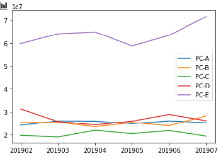
グラフ化
graph_data = pd.pivot_table(join_data, index='payment_month', columnst='item_name', values='price', aggfunc=''sum)
graph_data.head()
import matplotlib.pyplot as plt
%matplotlib inline
plt.plot(list(graph_data.index), graph_data["PC-A"], label='PC-A')
plt.plot(list(graph_data.index), graph_data["PC-B"], label='PC-B')
plt.plot(list(graph_data.index), graph_data["PC-C"], label='PC-C')
plt.plot(list(graph_data.index), graph_data["PC-D"], label='PC-D')
plt.plot(list(graph_data.index), graph_data["PC-E"], label='PC-E')
plt.legend()